Saturn’s Hexagon Is A Hexagonal Cloud Pattern That Has Persisted At The North Pole Of Saturn Since

In the garden. Värmland, Sweden (October 23, 2015).

Jupiter’s Galilean Moons

Io - Jupiter’s volcanic moon

Europa -  Jupiter’s icy moon

Ganymede - Jupiter’s (and the solar system’s) largest moon

Callisto -  Jupiter’s heavily cratered moon

Made using: Celestia, Screen2Gif & GIMP Based on: @spaceplasma‘s solar system gifs Profile sources: http://solarsystem.nasa.gov/planets, http://nssdc.gsfc.nasa.gov/planetary/factsheet/joviansatfact.html

Mathematics is full of wonderful but “relatively unknown” or “poorly used” theorems. By “relatively unknown” and “poorly used”, I mean they are presented and used in a much more limited scope than they could be, so the theorem may be well known, but only superficially, and its generality and scope can be very understated and underappreciated.

One of my favorites of such theorems was discovered around the 4th century by the Greek mathematician Pappus of Alexandria. It is known as Pappus’s Centroid Theorem.

Pappus’s theorem originally dealt with solids of revolution and their surface areas and volumes. This was all Pappus was able to figure out with the geometric proof methods available to him at the time. Later on, the theorem was rediscovered by Guldin, and studied by Leibniz, Cavalieri and Euler.

The theorem is usually split into two, one for areas and one for volumes. However, the basic principle that makes both work is exactly the same, though it is much more general in the case of areas on a plane, or volumes in space.

The invention/discovery of calculus eventually brought to the table much more general methods that made Pappus’s theorem somewhat limited in comparison.

Still, the theorem is based on a very clever idea that is quite satisfying both conceptually and intuitively, and brilliant in its simplicity. By knowing this key idea one can greatly simplify some problems involving volumes and areas, so the theorem can still be useful, especially when associated with methods from calculus.

Virtually all of the literature that mentions the theorem focus on solids of revolution only, as if the theorem was merely a curiosity, and they never really address why centroids would play a role. This is a big shame. The theorem is much more general, useful and conceptually interesting, and that’s why I’m writing this long post about it. But first, a few words on centroids.

Centroids

Centroids are the purely geometric analogues of centers of mass. They are a single point, not necessarily lying inside a shape, that defines the weighted “average position” of a shape in space. Naturally, the center of mass of any physical object with uniform density coincides with its geometric centroid, since the mass is uniformly distributed along the object’s volume.

Centers of mass are useful because they give you a point of balance: you can balance any object by any point directly under its center of mass (under constant vertical gravity). This comes from the fact the torques acting on the shape exactly cancel out in this configuration, so the object does not tilt either way.

Centroids exist for objects with any dimension you wish. A scattering of points has a centroid that is just their average position. In 1 dimension we have a line segment, whose centroid is always at its center. In 2, 3 or more dimensions, things get a bit trickier. We can always find the centroid by integrating all over the shape and weighting each point by that point’s position. This is generally a complicated enough problem by itself, but for simpler shapes this can be trivial.

Centroids, as well as centers of mass, also have the nice property of being additive: the union of two shapes has a centroid that is the weighted average of both centroids. So if you can decompose a shape into simpler ones, you can find its centroid without any hassle.

Pappus’s Centroid Theorems (for surfaces of revolution)

So, let’s imagine we have ourselves some generic planar curve, which we’ll call the generator. This can be a line segment or some arc of a circle, like in the main animation of this post, above. Anything will do, as long as it lies on a plane.

If we rotate the generator around an axis lying on its plane, and which does not cross the generator, it will “sweep” an area in space. Pappus’s theorem then states:

The surface area swept by a generator curve is equal to the length of the generator c multiplied by the length of the path traced by the geometric centroid of the generator L. That is: A = Lc.

In other words, if you have a generating curve with length c, and its centroid is at a distance a from the axis of rotation, then after a complete turn the generator will have swept an area A = 2πac, where L = 2πa is just the circumference of the circle traced by the centroid. This is what the first animation in this post is showing.

Note that in that animation we are ignoring the circular parts on top and bottom of the cylinder and cone, for simplicity. But this isn’t really a limitation of the theorem at all. If we add line segments for generating those regions we get a new generator with a different centroid, and the theorem still holds. Here’s what that setup looks like:

Try doing the math! It’s nice to see how things work out in the end.

The second theorem is exactly the same statement, but it deals with volumes. So, instead of a planar curve, we now have a closed planar shape with an area A.

If we now rotate it around an axis, the shape will sweep a volume in space. The volume is then just area of the generating shape times the length of the path traced by its centroid, that is, V = LA = 2πRA, where R is the distance the centroid is from the axis of rotation.

Why it works

Now, why does this work? What’s the big deal about the centroid? Here’s an informal, intuitive way to understand it.

You may have noticed that I drew the surfaces in the previous animations in a peculiar translucent way. This was done intentionally, not just to give the surfaces a physically “real” feel, but to illustrate the reason why the theorem works. (It also looks cooler!)

Here are the closed cylinder and cone after they were generated by a rotating curve:

Notice how the center of the top and bottom of the cylinder and the cone are a darker, denser color? This results from the fact that the generator is sweeping more “densely” in those regions. Farther out from the center of rotation, the surface is lighter, indicating a lower “density”.

To better convey this idea, let’s consider a line segment and a curve on a plane.

Below, we see equally spaced line segments of the same length placed along a red curve, perpendicular to it, in two different ways. Under the segments, we see the light blue area that would be swept by the line segment as it moved along the red curve in this way.

In this first case, the segments are placed with one edge on the curve. You can see that when the red curve bends, the spacing between the segments is not constant, since they are not always parallel to each other. This is what results in the different density in the “sweeping” of the surface’s area. Multiplying the length of those line segments by the length of the red curve will NOT give you the total area of the blue strip in this case, because the segments are not placed along the curve centered at their geometric centroids.

What this means is that the differences in areas being swept by the segment as the curve bends don’t cancel out, that is, the bits with more density don’t make up for the ones with a lower density, canceling out the effect of the bend.

However, in this second case, we place the segment so that its centroid is along the curve. In this case, the area is correctly given by Pappus’s theorem, because whenever there’s a bend in the curve one side of the segment is sweeping in a lower density and the other is sweeping at a higher density in a such a way that they both exactly cancel out.

This happens because that “density” is inversely proportional to the “speed” of each point of the line segment as it is moving along the red curve. But this “speed” is directly proportional to the distance to the point of rotation, which lies along the red curve.

Therefore, things only cancel out when you use the centroid as the anchor/pivot on the curve, which allows us to assume a constant density throughout the entire path, which in turn means there’s a constant area/volume being swept per unit of length traversed. The theorem follows directly from this result.

The same argument works in 3D for volumes.

Generalizations and caveats

As mentioned, the theorem is much more general than solids and surfaces of revolution, and in fact works for a lot of tracing curves (open or closed) and generators, as long as certain conditions are met. These are described in detail in the article linked at the end.

First, the tracing curve, the one where the generator moves along (always colored red in these illustrations), needs to be sufficiently smooth, otherwise you can’t properly define the movement of the generator along its extent. Secondly, the generator must be two dimensional, always lying on a plane perpendicular to the tracing curve. Third, in order for the theorem to remain simple, the curve and the plane must intersect at the centroid of the generator.

This means that, in two dimensions, the generator can only be a line segment (or pieces of it), as in the previous images. In this case, both the “2D volume” (the area) and “2D area” (the lateral curves that bound the area, traced by the ends of the segment) can be properly described by the theorem. If the tracing curve has sharp enough bends or crosses itself, then different regions may be covered more than once. This is something that needs to be accounted for via other means.

The immediate extension of this 2D case to 3D is perfectly valid as well, where the line segment gets replaced by a circle as a generator. This gives us a cylindrical tube of constant radius along the tracing curve in space, no longer confined to a plane. Both the lateral surface area of the tube and its volume can be computed directly by the theorem. You can even have knots as the curve!

In 3D, we could also have other shapes instead of a circle as the generator. In this case there are complications, mostly because now the orientation of the shape matters. Say, for example, that we have a square-shaped generator. As it moves along a curve it can also twist around, as seen in the animation below:

In both cases, the volume is exactly the same, and is given by Pappus’ theorem. This can be understood as a generalization of Cavalieri’s principle along the red curve, which also only works because we’re using the centroid as our anchor.

However, the surface areas in this case are NOT the same: the surface area of the twisted version is larger.

But if the tracing curve is planar (2D) itself and the generator does not rotate relative to the curve (that is, it remains “upright” all along the path), like in the case of surfaces of revolution, then the theorem works fine for areas in 3D.

So the theorem holds nicely for “2D volumes” (planar areas) and 3D volumes, but usually breaks down for surface areas in 3D. The theorem only holds for surface areas in 3D in a particular orientation of the generator along the curve (see reference).

In all valid cases, however, the centroid is the only point where you get the direct statement of the theorem as mentioned before.

Further generalizations

Since the theorem holds for 2D and 3D volumes, we can do a lot more with it. So far, we only considered a generator that is constant along the curve, which is why we have the direct expression for the volume. We actually don’t need this restriction, but then we have to use calculus.

For instance, in 3D, given a tracing curve parametrized by 0 ≤ s ≤ L, and a generator as a shape of area A(s), which varies along the curve in such a way that the centroid is always in the curve, then we can compute the total volume simply by evaluating the integral:

V = ∫0LA(s) ds

Which is basically a line integral along the scalar field given by A(s).

This means we can use Pappus theorem to find the volume of all sorts of crazy shapes along a curve in space, which is quite nifty. Think of tentacles, bent pyramids and crazy helices, like this one:

What we have here are five equal equilateral triangles positioned on the vertices of a regular pentagon. Their respective centroids lie on their centers, and since all of them have the same area the overall centroid (the blue dot) is exactly in the middle of the pentagonal shape, which is true no matter how you rotate the pentagon or the individual triangles.

This means we can generate a solid along the red curve by sweeping these triangles while everything rotates in any crazy way we want (like the overall pentagon and each individual triangle separately, as in the animation), and Pappus’s theorem will give us the volume of this shape just the same. (But not the area!)

If this doesn’t convince you this theorem is awesome and underappreciated, I don’t know what will.

So there you go. A nifty theorem that doesn’t get enough love and appreciation.

Reference

For a great, detailed and proper generalization of the theorem (which apparently took centuries to get enough attention of someone) see:

A. W. Goodman and Gary Goodman, The American Mathematical Monthly, Vol. 76, No. 4 (Apr., 1969), pp. 355-366. (You can read it for free online, you just need an account.)

Cosmic horseshoe is not the lucky beacon

A UC Riverside-led team of astronomers use observations of a gravitationally lensed galaxy to measure the properties of the early universe

Although the universe started out with a bang it quickly evolved to a relatively cool, dark place. After a few hundred thousand years the lights came back on and scientists are still trying to figure out why.

Astronomers know that reionization made the universe transparent by allowing light from distant galaxies to travel almost freely through the cosmos to reach us.

However, astronomers don’t fully understand the escape rate of ionizing photons from early galaxies. That escape rate is a crucial, but still a poorly constrained value, meaning there are a wide range of upper and lower limits in the models developed by astronomers.

That limitation is in part due to the fact that astronomers have been limited to indirect methods of observation of ionizing photons, meaning they may only see a few pixels of the object and then make assumptions about unseen aspects. Direct detection, or directly observing an object such as a galaxy with a telescope, would provide a much better estimate of their escape rate.

In a just-published paper, a team of researchers, led by a University of California, Riverside graduate student, used a direct detection method and found the previously used constraints have been overestimated by five times.

“This finding opens questions on whether galaxies alone are responsible for the reionization of the universe or if faint dwarf galaxies beyond our current detection limits have higher escape fractions to explain radiation budget necessary for the reionization of the universe,” said Kaveh Vasei, the graduate student who is the lead author of the study.

It is difficult to understand the properties of the early universe in large part because this was more than 12 billion year ago. It is known that around 380,000 years after the Big Bang, electrons and protons bound together to form hydrogen atoms for the first time. They make up more than 90 percent of the atoms in the universe, and can very efficiently absorb high energy photons and become ionized.

However, there were very few sources to ionize these atoms in the early universe. One billion years after the Big Bang, the material between the galaxies was reionized and became more transparent. The main energy source of the reionization is widely believed to be massive stars formed within early galaxies. These stars had a short lifespan and were usually born in the midst of dense gas clouds, which made it very hard for ionizing photons to escape their host galaxies.

Previous studies suggested that about 20 percent of these ionizing photons need to escape the dense gas environment of their host galaxies to significantly contribute to the reionization of the material between galaxies.

Unfortunately, a direct detection of these ionizing photons is very challenging and previous efforts have not been very successful. Therefore, the mechanisms leading to their escape are poorly understood.

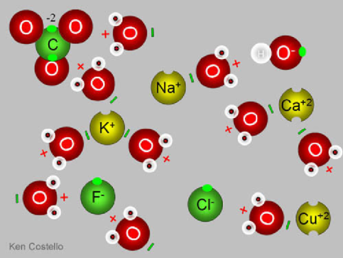
This has led many astrophysicists to use indirect methods to estimate the fraction of ionizing photons that escape the galaxies. In one popular method, the gas is assumed to have a “picket fence” distribution, where the space within galaxies is assumed to be composed of either regions of very little gas, which are transparent to ionizing light, or regions of dense gas, which are opaque. Researchers can determine the fraction of each of these regions by studying the light (spectra) emerging from the galaxies.

In this new UC Riverside-led study, astronomers directly measured the fraction of ionizing photons escaping from the Cosmic Horseshoe, a distant galaxy that is gravitationally lensed. Gravitational lensing is the deformation and amplification of a background object by the curving of space and time due to the mass of a foreground galaxy. The details of the galaxy in the background are therefore magnified, allowing researchers to study its light and physical properties more clearly.

Based on the picket fence model, an escape fraction of 40 percent for ionizing photons from the Horseshoe was expected. Therefore, the Horseshoe represented an ideal opportunity to get for the first time a clear, resolved image of leaking ionizing photons to help understand the mechanisms by which they escape their host galaxies.

The research team obtained a deep image of the Horseshoe with the Hubble Space Telescope in an ultraviolet filter, enabling them to directly detect escaping ionizing photons. Surprisingly, the image did not detect ionizing photons coming from the Horseshoe. This team constrained the fraction of escaping photons to be less than 8 percent, five times smaller than what had been inferred by indirect methods widely used by astronomers.

“The study concludes that the previously determined fraction of escaping ionizing radiation of galaxies, as estimated by the most popular indirect method, is likely overestimated in many galaxies,” said Brian Siana, co-author of the research paper and an assistant professor at UC Riverside.

“The team is now focusing on direct determination the fraction of escaping ionizing photons that do not rely on indirect estimates.”

Drops of a liquid can often join a pool gradually through a process known as the coalescence cascade (top left). In this process, a drop sits atop a pool, separated by a thin air layer. Once that air drains out, contact is made and part of the drop coalesces. Then a smaller daughter droplet rebounds and the process repeats.

A recent study describes a related phenomenon (top right) in which the coalescence cascade is drastically sped up through the use of surfactants. The normal cascade depends strongly on the amount of time it takes for the air layer between the drop and pool to drain. By making the pool a liquid with a much greater surface tension value than the drop, the researchers sped up the air layer’s drainage. The mismatch in surface tension between the drop and pool creates an outward flow on the surface (below) due to the Marangoni effect. As the pool’s liquid moves outward, it drags air with it, thereby draining the separating layer more quickly. The result is still a coalescence cascade but one in which the later stages have no rebound and coalesce quickly. (Image and research credit: S. Shim and H. Stone, source)

Transit of Venus

js

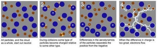
How Do Volcanoes Make Lightning?

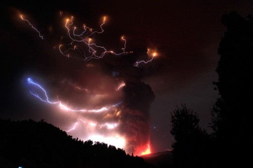
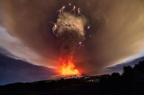
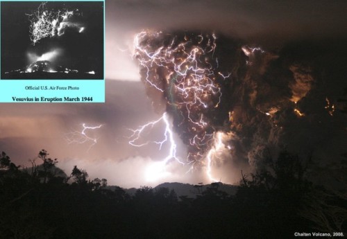
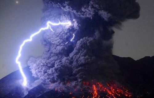
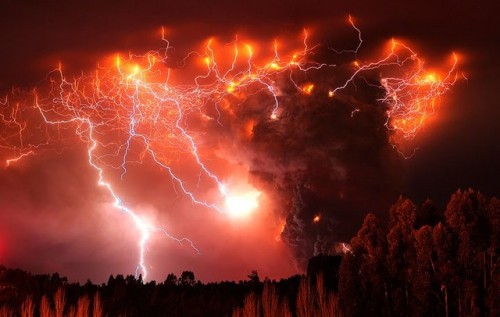
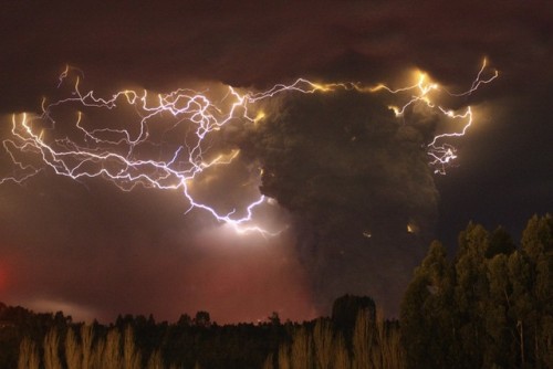
“Volcanic lightning appears to occur most frequently around volcanoes with large ash plumes, particularly during active stages of the eruption, where flowing, molten lava creates the largest temperature gradients. The phenomena of lightning has been exquisitely recorded around a number of recent volcanic eruptions, including Iceland’s Eyjafjallajökull, Japan’s Sakurajima, Italy’s Mt. Etna, and Chile’s Puyehue, Calbuco and Chaiten volcanoes. But what you may not know is this phenomenon was not only captured during Mt. Vesuvius’ last eruption in 1944, but was accurately described nearly 2,000 years ago when it erupted all the way back in the year 79!”

Volcanoes are some of the most potentially destructive natural phenomena known to occur on our world. The most violent eruptions feature not only lava, but soot, ash, volatile gases, and even enormous chunks of rock hurled great distances. What you might not realize, however, is just how frequently these eruptions are accompanied by another spectacular show: volcanic lightning. Lightning isn’t only found in thunderstorms or other great electrical discharges between the clouds and the ground, but is produced in volcanic eruptions all throughout the world, and throughout history as well. After countless generations, where we wondered what could produce such an unusual but spectacular show, we’ve finally figured it out.

Come get the science behind how volcanoes make lightning, and enjoy some of the greatest photographs of this phenomena humanity’s ever taken!

Anticrepuscular Rays Over Florida

White jellyfish by Alberto Montalesi Via Flickr: